Formatting cells in Excel is essential for improving readability and presentation. You can customize various aspects of cell formatting, including font styles, sizes, colors, and more. Here’s how you can format cells for better readability:
Font Styles, Sizes, and Colors:
- Changing Font Style:
- Select the cell or range of cells you want to format.
- Go to the “Home” tab on the Excel ribbon.
- In the “Font” group, use the dropdown menus to select the desired font style.
- Changing Font Size:
- Select the cell or range of cells you want to format.
- Go to the “Home” tab on the Excel ribbon.
- In the “Font” group, use the dropdown menu to select the desired font size.
- Changing Font Color:
- Select the cell or range of cells you want to format.
- Go to the “Home” tab on the Excel ribbon.
- In the “Font” group, click on the “Font Color” button to choose a color.
Cell Background Color:
- Changing Cell Background Color:
- Select the cell or range of cells you want to format.
- Go to the “Home” tab on the Excel ribbon.
- In the “Font” group, click on the “Fill Color” button to choose a background color for the selected cells.
Applying Cell Borders:
- Adding Cell Borders:
- Select the cell or range of cells you want to format.
- Go to the “Home” tab on the Excel ribbon.
- In the “Font” group, click on the “Borders” dropdown button.
- Choose the desired border style, such as “All Borders” or specific border options.
Applying Number Formatting:
- Number Formatting:
- Select the cell or range of cells containing numbers.
- Go to the “Home” tab on the Excel ribbon.
- In the “Number” group, use the dropdown menu to choose a number format, such as Currency, Date, Percentage, etc.
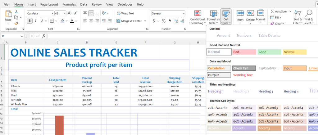
Applying Cell Styles:
- Using Cell Styles:
- Select the cell or range of cells you want to format.
- Go to the “Home” tab on the Excel ribbon.
- In the “Styles” group, click on the “Cell Styles” dropdown button.
- Choose a predefined cell style from the list, or click on “New Cell Style” to create a custom style.
Conditional Formatting:
- Conditional Formatting:
- Select the cell or range of cells you want to format conditionally.
- Go to the “Home” tab on the Excel ribbon.
- In the “Styles” group, click on “Conditional Formatting” and choose the desired formatting rule from the dropdown menu.
By using these formatting options, you can enhance the appearance of your Excel worksheets and make your data more visually appealing and easier to understand.