Sample Dataset:
Consider a dataset with student information where we want to retrieve the grades based on the student’s ID. Here’s a simplified version of the data:
| Student ID | Name | Grade |
|---|---|---|
| 101 | Alice | A |
| 102 | Bob | B |
| 103 | Charlie | C |
| 104 | David | B |
| 105 | Emma | A |
VLOOKUP Example:
Suppose we want to find the grade for a student with ID 103.
- Syntax:
=VLOOKUP(lookup_value, table_array, col_index_num, [range_lookup])- Parameters:
lookup_value: 103 (Student ID we want to look up)table_array: Range of cells containing the data (A1:C6)col_index_num: Column number containing the grades (3)range_lookup: FALSE (for exact match)
- Formula:
=VLOOKUP(103, A1:C6, 3, FALSE)- Result: The formula returns “C” as the grade for the student with ID 103.
XLOOKUP Example:
Now, let’s find the grade of the student with the name “Emma”.
- Syntax:
=XLOOKUP(lookup_value, lookup_array, return_array, [if_not_found], [match_mode], [search_mode])- Parameters:
lookup_value: “Emma” (Name of the student we want to look up)lookup_array: Range of cells containing the student names (B2:B6)return_array: Range of cells containing the grades (C2:C6)[if_not_found]: Optional parameter (we’ll leave it out for simplicity)[match_mode]: Optional parameter (defaults to 0, meaning exact match)[search_mode]: Optional parameter (defaults to 1, meaning search first to last)
- Formula:
=XLOOKUP("Emma", B2:B6, C2:C6)- Result: The formula returns “A” as the grade for the student named “Emma”.
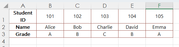
In this structure, the student IDs are in the first row and the corresponding grades are in the second row.
HLOOKUP Example with Different Data Structure:
Now, let’s find the grade of the student with ID 104 using HLOOKUP.
- Syntax:
=HLOOKUP(lookup_value, table_array, row_index_num, [range_lookup]) - Parameters:
lookup_value: 104 (Student ID we want to look up)table_array: Range of cells containing the data (A1:F2)row_index_num: Row number containing the grades (2, since grades are in the second row)range_lookup: FALSE (for exact match)
- Formula:
=HLOOKUP(104, A1:F2, 2, FALSE) - Result: The formula returns “B” as the grade for the student with ID 104.
Explanation:
In this example, the HLOOKUP function searches for the student ID (104) in the first row (containing IDs) and returns the corresponding grade from the second row. The function operates similarly to the previous example but with a different data structure.
This demonstrates the flexibility of the HLOOKUP function, allowing you to perform horizontal lookups across rows instead of columns. It’s particularly useful when your data is organized in a different orientation, such as when the criteria you’re searching for are in the top row.
These examples illustrate how to use VLOOKUP, HLOOKUP, and XLOOKUP functions with the same dataset. Each function serves a different purpose but allows you to retrieve specific information based on given criteria. Let me know if you need further clarification!