Excel offers a range of formatting tools to help you organize data effectively. Here’s a breakdown of how you can use borders, shading, and alignment:
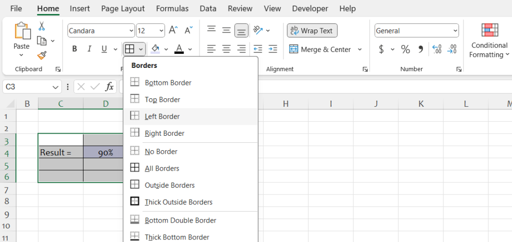
- Borders: Borders help to visually separate different sections of your data or highlight specific cells. To apply borders:
- Select the range of cells you want to format.
- Go to the “Home” tab on the Excel ribbon.
- In the “Font” group, you’ll find the “Borders” button. Click the drop-down arrow next to it to see different border styles.
- Choose the border style you want to apply, such as “All Borders,” “Outside Borders,” or “Thick Box Border.”

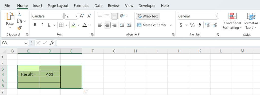
- Shading: Shading helps to differentiate between different parts of your data or to highlight specific cells. To apply shading:
- Select the range of cells you want to shade.
- Again, go to the “Home” tab on the Excel ribbon.
- In the “Font” group, you’ll find options for fill color. Click the drop-down arrow to choose a color, or select “More Fill Colors” for a wider range of options.
- Click on the desired color to apply it to the selected cells.

- Alignment: Proper alignment can make your data more readable and organized. To adjust alignment:
- Select the range of cells you want to align.
- Go to the “Home” tab on the Excel ribbon.
- In the “Alignment” group, you’ll find options for horizontal and vertical alignment, as well as text orientation.
- Click on the appropriate alignment buttons to align text left, center, or right horizontally, and top, middle, or bottom vertically.
- You can also use the alignment buttons to wrap text, merge cells, or rotate text to a specific angle.

By using these formatting tools effectively, you can make your Excel worksheets more visually appealing and easier to understand, which can improve readability and analysis.