Excel advanced functions like VLOOKUP, HLOOKUP, INDEX-MATCH, and SUMIFS are powerful tools in Excel for performing more complex calculations and data lookups. Here’s an overview of each:
- VLOOKUP (Vertical Lookup):
- VLOOKUP searches for a value in the first column of a table and returns a corresponding value in the same row from a specified column.
- Syntax:
=VLOOKUP(lookup_value, table_array, col_index_num, [range_lookup]) - Example formla on A4:
=VLOOKUP(A2, B:C, 2, FALSE)searches for the value in cell A2 in column B, and returns the corresponding value from column C. The last argument,[range_lookup], set to FALSE, ensures an exact match.

- HLOOKUP (Horizontal Lookup):
- HLOOKUP searches for a value in the first row of a table and returns a corresponding value in the same column from a specified row.
- Syntax:
=HLOOKUP(lookup_value, table_array, row_index_num, [range_lookup]) - Example formla on A4:
=HLOOKUP(A2, B1:G10, 5, FALSE)searches for the value in cell A2 in row 1, and returns the corresponding value from row 2. The last argument,[range_lookup], set to FALSE, ensures an exact match.

- INDEX-MATCH:
- INDEX-MATCH is a combination of the INDEX and MATCH functions, offering more flexibility and power compared to VLOOKUP.
- INDEX returns the value of a cell in a specific row and column of a table or range.
- MATCH searches for a specified value in a range and returns the relative position of that item.
- Syntax (INDEX):
=INDEX(array, row_num, [column_num]) - Syntax (MATCH):
=MATCH(lookup_value, lookup_array, [match_type]) - Example formla on A4:
=INDEX(B1:B6, MATCH(A2, C1:C6, 0))searches for the value in cell A2 in column B, and returns the corresponding value from column C.

- SUMIFS:
- SUMIFS adds the cells in a range that meet multiple criteria.
- Syntax:
=SUMIFS(sum_range, criteria_range1, criteria1, [criteria_range2, criteria2], ...) - Example formla on A4:
=SUMIFS(D:D, B:B, "Apples", C:C, ">10")sums the values in column D where the corresponding value in column B is “Apples” and the value in column C is greater than 10.

- IFERROR:
- IFERROR allows you to handle errors gracefully by specifying the value or action to take if a formula results in an error.
- Syntax:
=IFERROR(value, value_if_error) - Example:
=IFERROR(H8/G8, "Error: Division by zero")will return “Error: Division by zero” if there’s an error in the division.


- CHOOSE:
- CHOOSE returns a value from a list of values based on its position.
- Syntax:
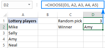
=CHOOSE(index_num, value1, [value2], ...) - Example:
=CHOOSE(D1, A2, A3, A4)returns “Mike” if D1 is 1, “Sally” if D1 is 2, and so on.

- TEXTJOIN:
- TEXTJOIN combines multiple text strings from a range into one text string, with an optional delimiter.
- Syntax:
=TEXTJOIN(delimiter, ignore_empty, text1, [text2], ...) - Example:
=TEXTJOIN(", ",TRUE,C3:C7)combines the text values in cells C3 to C7, separated by a comma and space.

- ARRAYFORMULA:
- ARRAYFORMULA is a Google Sheets function that doesn’t directly exist in Excel, but you can achieve similar functionality using array formulas in Excel.
- It allows you to apply a formula to an entire range of cells without having to copy it down manually.
- Example:
{=F3:F7*H3:H7}multiplies each corresponding cell in columns F and H from rows 3 to 7.

- OFFSET:
- OFFSET returns a reference offset from a starting cell or range of cells by a specified number of rows and columns.
- Syntax:
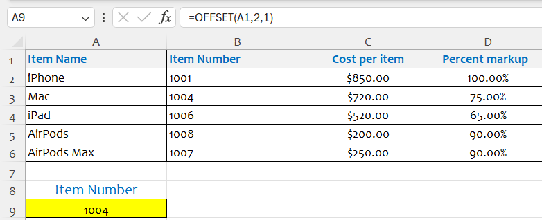
=OFFSET(reference, rows, cols, [height], [width]) - Example:
=OFFSET(A1, 2, 1)returns the value from the cell that is 2 rows down and 1 column to the right of cell A1.

These functions provide powerful tools for data manipulation and analysis in Excel, allowing you to perform complex lookups, matches, and calculations with ease. Understanding and mastering these functions can greatly enhance your productivity and effectiveness in working with Excel data.